

Following Friday’s announcement that real gross domestic product (GDP) grew by 4.1 percent (at a seasonally adjusted annual rate) in the most recent quarter, the business news was filled with stories about how big the number was.
Even the most casual reader of financial and economic news knows that the speed of economic growth matters. Businesses―manufacturers, service providers, and retailers, among others―need to know so that they can decide how much to invest in new production facilities, how many people to employ, and what to stock on their shelves. Fiscal policymakers need to know so that they can estimate government revenue and expenditure. And monetary policymakers need to know so that they can adjust their policies in an effort to ensure low, stable inflation and strong, stable, and balance growth.
But, does it make sense for all of these people―firms, households and governments―to focus on fresh estimates of GDP? How much attention should we pay to any new number? That is, when the U.S. Bureau of Economic Analysis (BEA) announces that their initial estimate of growth for the quarter just ended is 2% or 3% or (as it was last week) 4%, what should we think?
While GDP was once a key cyclical indicator, its value has declined substantially. In this post, we highlight three reasons: timeliness, seasonal adjustment and revisions. Not surprisingly, in the era of big data, those who need information on growth are increasingly turning to more timely indicators customized to their needs.
Timeliness. People in national statistical agencies that produce the GDP data―in the United States, these are the employees of the Bureau of Economic Analysis―are very good at their jobs. But, because of the delay in obtaining a broad swathe of information, they are slow. By the time we get the first estimate of GDP for a given three-month period―nearly a full month after the end of the quarter―we already have a myriad of indicators for the same period. We know employment, retail sales, industrial production, housing starts, motor vehicle sales, etc. etc. etc.
In fact, using ever faster computing technology, over the past decade econometricians have developed techniques to construct real-time estimates of aggregate economic activity. For U.S. GDP, the Federal Reserve Banks of Atlanta and New York produce competing nowcasts (see here and here). Since April, the Atlanta Fed’s GDPNow estimate had been within 0.5 percentage points of the 4.1% estimate published by the BEA at the end of July. Not surprisingly, from a financial market perspective, the GDP report carries little news.
Seasonality. The following chart plots GDP growth―quarterly at an annual rate―using the unadjusted (black line) and the conventionally reported seasonally adjusted (red line) series. This is a striking figure. First, note the vertical scale goes from –20 to +20 percent! Second, while the adjusted data shows some variability, the range is far smaller. The unadjusted data exhibits an enormous annual drop and rebound. Most people would be surprised to learn that the United States experiences a depression every winter and a boom every spring.
Seasonally adjusted and unadjusted quarter-to-quarter annualized GDP growth (percent),
2002 to 2Q 2018

Source: Bureau of Economic Analysis.
To see how big the depression is, we plot below the average size of the seasonal adjustment over the period since 2002 – the data that we have available. On average, statisticians add 14.4% to first quarter GDP and subtract 6.2% from fourth quarter GDP to get from the unadjusted to the adjusted data. This means that, from the fourth quarter to the first quarter, GDP typically plunges by 20.6% every year!
Average seasonal adjustment by quarter (percent), 2002 to 2Q 2018
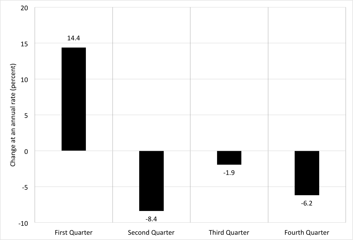
Source: Bureau of Economic Analysis and authors’ calculation.
It should be obvious that proper seasonal adjustment is critical to measure GDP growth accurately. As it turns out, however, it is an extremely difficult task. To understand why, consider how hard it is to adjust for variations in weather from year to year. Or, the fact that, since some producers face capacity constraints, seasonality tends to be less pronounced during booms. (See here and here.)
Seasonal adjustment is so difficult that, a few years ago, people noted that as a result of residual seasonality the seasonally adjusted data were understating first-quarter growth. In other words, the seasonal factor being added to first quarter GDP was too small. The most recent GDP benchmark revision published on Friday tries to take care of this problem.
Revisions. In an effort to improve their estimates, the BEA is constantly revising them. Not only do they obtain additional data―tax information, new census and survey results, and the like―but they also improve their methodology and introduce changes in various classifications.
On methods, the biggest challenge facing any national statistical office is the conversion of nominal quantities, which are relatively straightforward to measure, into inflation-adjusted real quantities. Doing this requires tools for measuring the quality of goods and services. When the price of a product goes up or down, statisticians need to decompose the change into the portion due to a change in quality and the part that is purely a price change. This is a challenging task, and one where methods are constantly improving. In some sectors, like health care, which now represents 17% of consumption, it is particularly difficulty to distinguish quality and price in order to measure inflation-adjusted expenditure (for a recent discussion, see here).
Regarding the classification of various activities and products, BEA must constantly decide whether something that is used in production is an intermediate input or an investment. The former doesn’t count in GDP, while the latter does. In recent years, various research and development (R&D) and software expenses have been reclassified as investment, substantially boosting measured GDP.
All of this means that revisions occur constantly and continue for decades! Take as an example the data for GDP in the second quarter of a given year. The initial estimate (like Friday’s release) is published at the end of July. Then for three succeeding months―in August, September and October―there are revisions. Every July for the next five years brings another set of revisions. And, every five years, there is a comprehensive update that goes back further: the most recent one released last week revised data back to 1929. (For a description of what was changed in the 2018 update, see here.)
You might think that these updates are small, but they are not. The changes from the initial estimate to the latest reading average 1.3% (without regard to sign), with a standard deviation of 1.0% (see here). And, the changes tend to be especially large around business cycle turning points—that is, when a recession is starting or ending—precisely when high-frequency cyclical information is particularly needed. To see this, we have picked an (admittedly extreme) example: the third quarter of 1990. Using the real-time data set of the Federal Reserve Bank of Philadelphia, we constructed the following chart of the progression of estimates of quarterly growth (at a seasonally adjusted annual rate) for the third quarter of 1990 from initial release in October 1990 to the current estimate to the most recent published on July 27, 2018.
Revisions to Third Quarter 1990 GDP Growth, 1990 to 2018
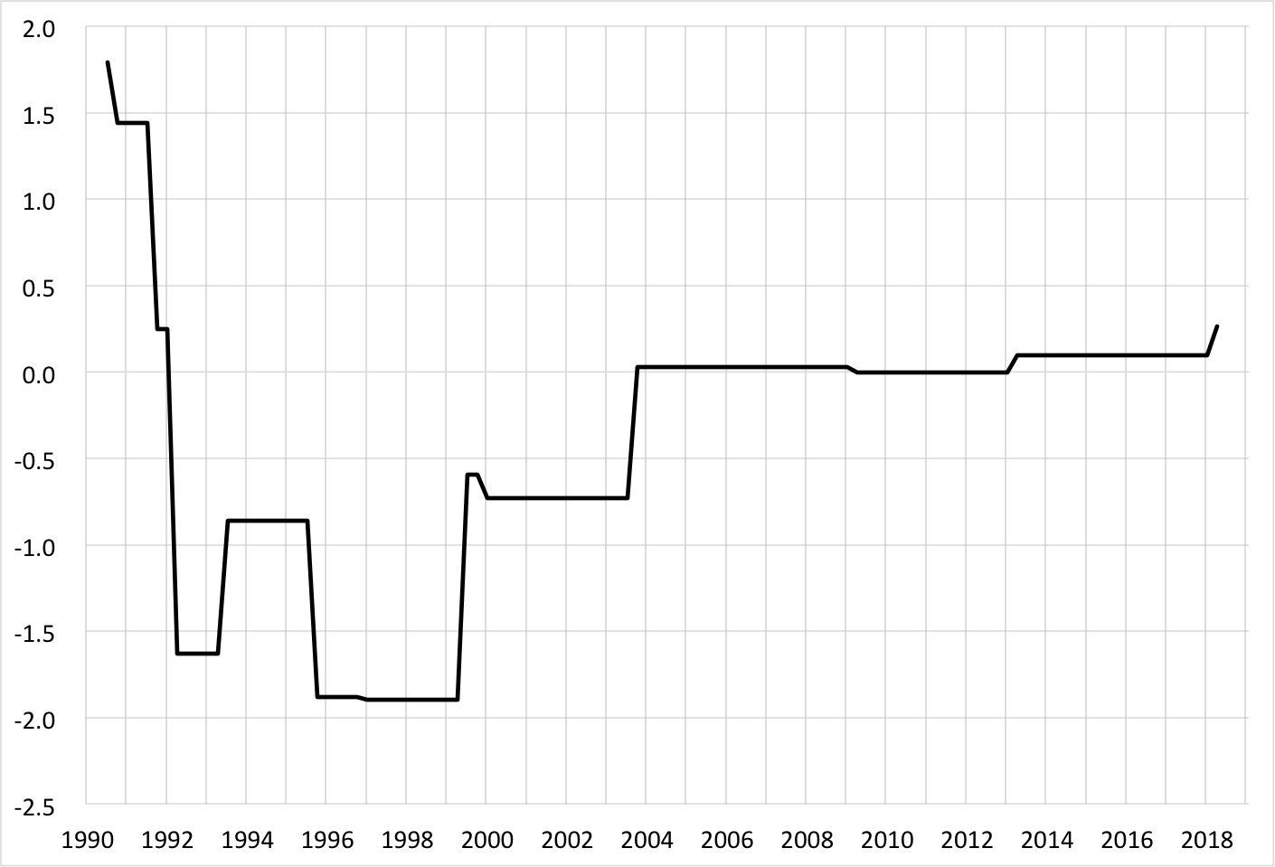
Source: Bureau of Economic Analysis and Federal Reserve Bank of Philadelphia.
Looking at the chart, we can see that the initial estimate (published in October 1990) suggested that the economy had grown by +1.8%. Since the economy was not doing well at the time, this came as welcome news. But, as the revisions rolled in, the story changed dramatically: by mid-1992, the estimate was down to –1.6%. As the chart shows, this was far from the end of the story. The mid-2003 revision―a full 13 years after the event―moved the estimate to zero. This is where things have roughly stayed. That is, until July 2018 when there was an upward revision. So, 28 years after the fact, we now believe that during April to June 1990 the economy grew by one-quarter of one percent.
The third quarter of 2008—at the height of the financial crisis—is another stark case involving dramatic revisions. Estimates of the economic collapse following the Lehman bankruptcy in 2008 were initially much too optimistic, showing a roughly 4 percent contraction. This was revised almost immediately to less than –5%. But it took three years, until mid-2011, for the estimate to go below –8%, where it has stayed. By that time, the economy was well into the current recovery, far too late to revise monetary or fiscal policy to stabilize activity.
So, this leads us to conclude that we should not put too much stock in early estimates of GDP. They will surely change. And, if something dramatic is happening, then the revisions can be large.
As an aside, it is worth noting that refinements not only influence short-run fluctuations, they can also change long-run trends. Using past vintages of GDP, we can see that growth estimates have slowly increased over time. For example, looking at the first decade of this century, in 2013 we thought average annual growth from 2001 to 2010 was 1.53%. With the most recent revision, we now believe the number was 1.74%―an increase of 0.2% per year. This does not change our view that growth since 2000 has been roughly half what it was in the prior quarter century, but it does constitute a material change. Similarly, the latest accounts show large increases since 2012 in the estimated personal savings rate—including a doubling of the 2017 estimate from 3.4% to 6.7%.
Conclusion. What should we make of all this? We draw two conclusions. First, quarterly changes in GDP are extremely noisy. And our initial estimates are even noisier. So, politicians’ and journalists’ taste for the immediate notwithstanding, it makes little sense to pay close attention.
However, people need guides about economic performance. Firms, households and governments make decisions based on their views of the future. In practice, however, they probably need something different from a measure like GDP. A firm producing cars needs a different set of information from one selling pizzas. And governments in different locales need data that is specific to their region. So, while GDP has provided an incredibly useful service since it was invented in the 1930s, people already are looking to a range of alternatives. Put differently, now that we have timely access to enormous amounts of raw data about consumption, investment, production and the like, a lagging summary statistic like GDP seems less useful.
An analogy to the pharmaceutical industry seems apt here: medical researchers are in the process of harnessing modern genetic technology to develop individually-tailored drug therapies. Over time, we probably will do something similar for economic indicators: employ the combination of analytic tools, cheap computing power and large data sets to develop custom economic indicators designed to address narrow questions. In the limit, perhaps we will each have our own measure of economic activity that is appropriate for what we do.
Surely, one size no longer fits all.